MVA 2018-19
To download this notebook or its pdf version:
http://geometrica.saclay.inria.fr/team/Fred.Chazal/MVA2018.html
Documentation for the latest version of Gudhi:
Simplicial complexes and simplex trees
In Gudhi, (filtered) simplicial complexes are encoded through a data structure called simplex tree. Here is a very simple example illustrating the use of simplex tree to represent simplicial complexes. See the Gudhi documentation for a complete list of functionalities. Try the following code and a few other functionalities from the documentation to get used to the Simplex Tree data structure.
import numpy as np
import gudhi as gd
import random as rd
import matplotlib.pyplot as plt
st = gd.SimplexTree() # Create an empty simplicial complex

# Simplicies can be inserted 1 by 1
# Vertices are indexed by integers
if st.insert([0,1]):
    print("First simplex inserted!")
st.insert([1,2])
st.insert([2,3])
st.insert([3,0])
st.insert([0,2])
st.insert([3,1])
L = st.get_filtration() # Get a list with all simplices
# Notice that inserting an edge automatically inserts its vertices, if they were not already in the complex
for simplex in L:
    print(simplex)
# Insert the 2-skeleton, giving some filtration values to the faces
st.insert([0,1,2],filtration=0.1)
st.insert([1,2,3],filtration=0.2)
st.insert([0,2,3],filtration=0.3)
st.insert([0,1,3],filtration=0.4)

# If you add a new simplex with a given filtration value, all its faces that
# were not in the complex are inserted with the same filtration value
st.insert([2,3,4],filtration=0.7)
st.get_filtration()
# Many operations can be done on simplicial complexes, see also the Gudhi documentation and examples
print("dimension=",st.dimension())
print("filtration[1,2]=",st.filtration([1,2]))
print("filtration[4,2]=",st.filtration([4,2]))
print("num_simplices=", st.num_simplices())
print("num_vertices=", st.num_vertices())
print("skeleton[2]=", st.get_skeleton(2))
print("skeleton[1]=", st.get_skeleton(1))
print("skeleton[0]=", st.get_skeleton(0))
Filtrations and persistence diagrams
# As an example, we assign to each simplex its dimension as filtration value
for splx in st.get_filtration():
    st.assign_filtration(splx[0],len(splx[0])-1)
# Let the structure know that we have messed with it and an old filtration cache may be invalid.
# This is redundant here because get_filtration() does it anyway, but not all functions do.
st.initialize_filtration()
st.get_filtration()
# To compute the persistence diagram of the filtered complex
# By default it stops at dimension-1, use persistence_dim_max=True
# to compute homology in all dimensions
diag = st.persistence(persistence_dim_max=True)
# Display each interval as (dimension, (birth, death))
print(diag)
# Plot a persistence diagram
gd.plot_persistence_diagram(diag)
gd.plot_persistence_barcode(diag)
# To compute the bottleneck distance between diagrams
st2 = gd.SimplexTree()
st2.insert([0,1],filtration=0.0)
st2.insert([1,2],filtration=0.1)
st2.insert([2,0],filtration=0.2)
st2.insert([0,1,2],filtration=0.5)
diag2 = st2.persistence()
gd.plot_persistence_diagram(diag2)
diag_0 = st.persistence_intervals_in_dimension(0)
diag2_0 = st2.persistence_intervals_in_dimension(0)
dB0 = gd.bottleneck_distance(diag_0, diag2_0)

diag_1 = st.persistence_intervals_in_dimension(1)
diag2_1 = st2.persistence_intervals_in_dimension(1)
dB1 = gd.bottleneck_distance(diag_1, diag2_1)

print("bottleneck distance in dimension 0:", dB0)
print("bottleneck distance in dimension 1:", dB1)
Exercise
- Recall the torus is homeomorphic to the surface obtained by identifying the opposite sides of a square as illustrated below.
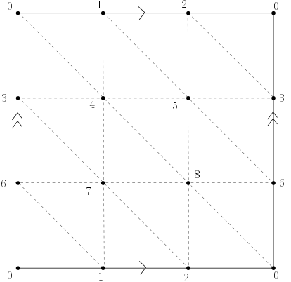 Using Gudhi, construct a triangulation (2-dimensional simplicial complex) of the Torus. Define a filtration on it, compute its persistence and use it to deduce the Betti numbers of the torus (check that you get the correct result using the function betti_numbers()).
 - Use Gudhi to compute the Betti numbers of a sphere of dimension 2 and of a sphere of dimension 3 (hint: the k -dimensional sphere is homeomorphic to the boundary of a (k+1)-dimensional simplex.
Stability of persistence for functions
The goal of this exercise is to illustrate the persistence stability theorem for functions on a very simple example. The code below allows to define a simplicial complex (the so-called α-complex) triangulating a set of random points in the unit square in the plane. Although we are not using it for this course, note that gudhi also provides the grid-like CubicalComplex, which may be a more natural choice to represent a function on a square.
n_pts=1000
# Build a random set of points in the unit square
X = np.random.rand(n_pts, 2)
# Compute the alpha-complex filtration
alpha_complex = gd.AlphaComplex(points=X)
st = alpha_complex.create_simplex_tree()
Let $p_0=(0.25, 0.25)$ and $p_1=(0.75, 0.75)$ be 2 points in the plane $\mathbb{R}^2$ and $\sigma=0.05$.
- Build on such a complex the sublevelset filtration of the function $$f(p)=\exp(-\frac{\|p-p_0\|^2}{\sigma})+3\exp(-\frac{\|p-p_1\|^2}{\sigma})$$ and compute its persistence diagrams in dimensions 0 and 1.
- Compute the persistence diagrams of random perturbations of f and compute the Bottleneck distance between these persistence diagrams and the perturbated ones. Verify that the persistence stability theorem for functions is satisfied.
Vietoris-Rips and alpha-complex filtrations
These are basic instructions to build Vietoris-Rips and α-complex filtrations and compute their persistence.
#Create a random point cloud in 3D
nb_pts=100
pt_cloud = np.random.rand(nb_pts,3)
#Build Rips-Vietoris filtration and compute its persistence diagram
rips_complex = gd.RipsComplex(pt_cloud,max_edge_length=0.5)
simplex_tree = rips_complex.create_simplex_tree(max_dimension=3)
print("Number of simplices in the V-R complex: ",simplex_tree.num_simplices())
diag = simplex_tree.persistence(homology_coeff_field=2, min_persistence=0)
gd.plot_persistence_diagram(diag).show()
#Compute Rips-Vietoris filtration and compute its persistence diagram from
#a pairwise distance matrix
dist_mat = []
for i in range(nb_pts):
    ld = []
    for j in range(i):
        ld.append(np.linalg.norm(pt_cloud[i,:]-pt_cloud[j,:]))
    dist_mat.append(ld)
rips_complex2 = gd.RipsComplex(distance_matrix=dist_mat,max_edge_length=0.5)
simplex_tree2 = rips_complex2.create_simplex_tree(max_dimension=3)
diag2 = simplex_tree2.persistence(homology_coeff_field=2, min_persistence=0)
gd.plot_persistence_diagram(diag2).show()
#Compute the alpha-complex filtration and compute its persistence
alpha_complex = gd.AlphaComplex(points=pt_cloud)
simplex_tree3 = alpha_complex.create_simplex_tree()
print("Number of simplices in the alpha-complex: ",simplex_tree3.num_simplices())
diag3 = simplex_tree3.persistence(homology_coeff_field=2, min_persistence=0)
gd.plot_persistence_diagram(diag3)
Exercise
- Illustrate the stability theorem for persistence diagrams of Vietoris-Rips and α-complex filtrations (take into accound that AlphaComplex uses the square of distances as filtration values).
- What happens to Vietoris-Rips and α-complex filtrations when the size of the point cloud increases? When the ambient dimension increases?