The goal of this lab session is to introduce ourselves to TDA using the R language and its package TDA, which uses the C++ library Gudhi as a backend.
We will use the following documents from the TDA Package:
Before you start, please refer to this page to install and configure R. Note that you will need R version 3.1.0 or higher to be able to install and run the TDA package.
To run R, simply type R in a terminal. You can write and execute commands in the R environment directly, or in dedicated source files (whose names should have the .R extension). To run a source file file.R in R, simply type source('file.R') in the R environment. To edit and execute source files you can use Emacs together with the ESS extension. Alternatively, you can use a dedicated IDE such as R-Studio. The choice of a particular IDE is always a matter of personal taste...
We will use the following packages:
The R command to know which packages are installed is library(). To use package pkg, just type library(pkg). The package must be installed in order to be used. The command to install the package is install.packages("pkg", dependencies = TRUE). The installation itself requires an access to the Internet. It downloads either source or binary files, depending on your OS and architecture. In case source files are downloaded (which is the case of the TDA package), you need to have make and a C++ compiler like gcc installed to compile the package. Please refer to the dedicated webpage for more information, and note that some OSes like Linux conveniently allow you to install packages globally (i.e. for all users) through their own package manager.To familiarize yourself with the basics of the R language, you can follow a tutorial such as this one (you can restrict yourself to the "R introduction" section, i.e. the introductory page and the pages on basic data types).
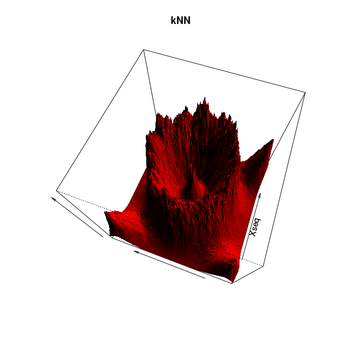
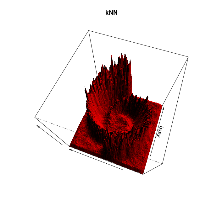
Follow Section 2.0 of the TDA package's tutorial. This section is about distance functions and density estimators. It ends right before Section 2.1 on bootstrap and confidence bands. To save time you may restrict yourself to the k nearest neighbor (kNN) density estimator.
Adapt then your code to compute and plot the kNN density estimator for the following 2d data sets: crater and spirals. You can use the command plot to plot the data.
Here is a solution and some pretty pictures (click on an image to see it at full resolution):
|
|
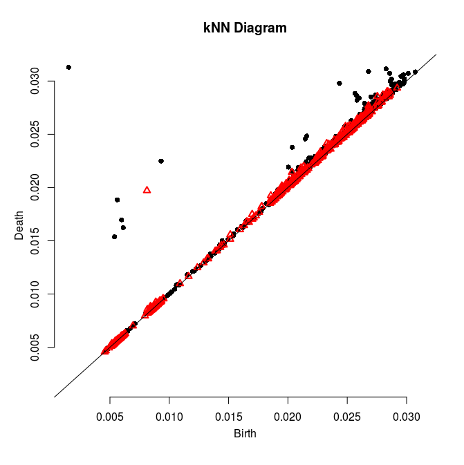
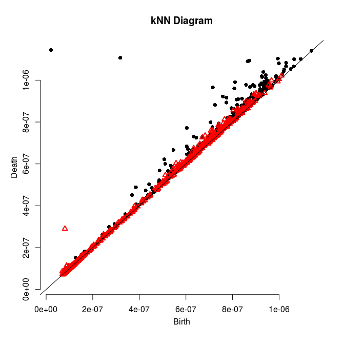
Follow Section 3.1 of the tutorial. This section is about computing persistence on a 2d grid.
Adapt then your code so that it computes the persistence diagram of the kNN density estimator. Check the validity of the output given what you know about the data.
Here is a solution and some pretty pictures (click on an image to see it at full resolution):
|
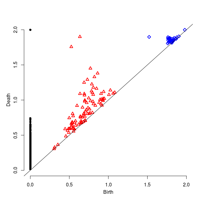
Follow now Section 3.2 of the tutorial. This section is about building Rips filtrations from point cloud data and computing their persistence diagram.
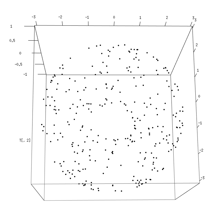
Generate now new data sets using the sphereUnif and torusUnif functions (please refer to the user's documentation of the TDA package for the details). Visualize the data using the plot3d command (from the rgl package) then compute their Rips filtrations and associated persistence barcodes. For this you will need to set the parameters carefully. Check the validity of the results given what you know about the data.
Here is a solution and some pretty pictures (click on an image to see it at full resolution):

|

|