R-TDA package tutorial
Mathieu Carrière and Steve Oudot
(adapted from the following tutorial by F. Chazal and B. Michel)
July 2016
For this practical lesson about Persistence Homology Inference, we need the TDA R-package.
install.packages("TDA", dependencies=TRUE) library(TDA) Persistence diagrams for Rips filtration
The ripsDiag() function computes the persistence diagram of the Rips filtration built on top of a point cloud.
The following code generates 60 points from two circles:
Circle1 <- circleUnif(60)
Circle2 <- circleUnif(60, r = 2) + 3
Circles <- rbind(Circle1, Circle2)
plot(Circles, pch = 16, xlab = "",ylab = "")
We specify the limit of the Rips filtration and the max dimension of the homological features we are interested in (0 for components, 1 for loops, 2 for voids, etc.).
maxdimension <- 1    # components and loops
maxscale <- 5        # limit of the filtration
and we generate the persistence diagram using either the C++ library GUDHI (or Dionysus):
Diag <- ripsDiag(X = Circles,
                 maxdimension,
                 maxscale,
                 library = "GUDHI",
                 printProgress = FALSE)
print(Diag[["diagram"]])
## dimension Birth Death
## [1,] 0 0.0000000 5.000000000
## [2,] 0 0.0000000 1.248655167
## [3,] 0 0.0000000 0.681882543
## [4,] 0 0.0000000 0.626945491
## [5,] 0 0.0000000 0.605573483
## [6,] 0 0.0000000 0.558305002
## [7,] 0 0.0000000 0.503336136
## [8,] 0 0.0000000 0.454175829
## [9,] 0 0.0000000 0.420407057
## [10,] 0 0.0000000 0.419658105
## [11,] 0 0.0000000 0.370848708
## [12,] 0 0.0000000 0.364224499
## [13,] 0 0.0000000 0.351474017
## [14,] 0 0.0000000 0.345539414
## [15,] 0 0.0000000 0.335991622
## [16,] 0 0.0000000 0.334634177
## [17,] 0 0.0000000 0.326365159
## [18,] 0 0.0000000 0.323037978
## [19,] 0 0.0000000 0.315383629
## [20,] 0 0.0000000 0.310536467
## [21,] 0 0.0000000 0.310262665
## [22,] 0 0.0000000 0.299689810
## [23,] 0 0.0000000 0.299347715
## [24,] 0 0.0000000 0.281637584
## [25,] 0 0.0000000 0.280511260
## [26,] 0 0.0000000 0.267956666
## [27,] 0 0.0000000 0.262500366
## [28,] 0 0.0000000 0.252993717
## [29,] 0 0.0000000 0.234222336
## [30,] 0 0.0000000 0.232796821
## [31,] 0 0.0000000 0.231153192
## [32,] 0 0.0000000 0.220700648
## [33,] 0 0.0000000 0.206815991
## [34,] 0 0.0000000 0.205821198
## [35,] 0 0.0000000 0.193307118
## [36,] 0 0.0000000 0.186722979
## [37,] 0 0.0000000 0.185064513
## [38,] 0 0.0000000 0.182864067
## [39,] 0 0.0000000 0.174142457
## [40,] 0 0.0000000 0.173349233
## [41,] 0 0.0000000 0.165982732
## [42,] 0 0.0000000 0.165499845
## [43,] 0 0.0000000 0.162600742
## [44,] 0 0.0000000 0.158470316
## [45,] 0 0.0000000 0.156601404
## [46,] 0 0.0000000 0.154588033
## [47,] 0 0.0000000 0.151872929
## [48,] 0 0.0000000 0.143354811
## [49,] 0 0.0000000 0.142104999
## [50,] 0 0.0000000 0.136520367
## [51,] 0 0.0000000 0.130379191
## [52,] 0 0.0000000 0.129089764
## [53,] 0 0.0000000 0.127437449
## [54,] 0 0.0000000 0.126321858
## [55,] 0 0.0000000 0.123633581
## [56,] 0 0.0000000 0.115843530
## [57,] 0 0.0000000 0.111836441
## [58,] 0 0.0000000 0.109250181
## [59,] 0 0.0000000 0.105035804
## [60,] 0 0.0000000 0.103326846
## [61,] 0 0.0000000 0.097845406
## [62,] 0 0.0000000 0.096205648
## [63,] 0 0.0000000 0.093575941
## [64,] 0 0.0000000 0.090009959
## [65,] 0 0.0000000 0.089763367
## [66,] 0 0.0000000 0.087647752
## [67,] 0 0.0000000 0.085860423
## [68,] 0 0.0000000 0.080253095
## [69,] 0 0.0000000 0.078960989
## [70,] 0 0.0000000 0.070546775
## [71,] 0 0.0000000 0.068519479
## [72,] 0 0.0000000 0.066857388
## [73,] 0 0.0000000 0.066597194
## [74,] 0 0.0000000 0.066324402
## [75,] 0 0.0000000 0.065312852
## [76,] 0 0.0000000 0.058724720
## [77,] 0 0.0000000 0.058459910
## [78,] 0 0.0000000 0.058093939
## [79,] 0 0.0000000 0.057353007
## [80,] 0 0.0000000 0.056634495
## [81,] 0 0.0000000 0.055391002
## [82,] 0 0.0000000 0.054714317
## [83,] 0 0.0000000 0.053954024
## [84,] 0 0.0000000 0.053309793
## [85,] 0 0.0000000 0.051547687
## [86,] 0 0.0000000 0.046986251
## [87,] 0 0.0000000 0.046791021
## [88,] 0 0.0000000 0.044507936
## [89,] 0 0.0000000 0.042748403
## [90,] 0 0.0000000 0.041996189
## [91,] 0 0.0000000 0.035464877
## [92,] 0 0.0000000 0.034858018
## [93,] 0 0.0000000 0.033600787
## [94,] 0 0.0000000 0.032788605
## [95,] 0 0.0000000 0.032157741
## [96,] 0 0.0000000 0.032049281
## [97,] 0 0.0000000 0.026104314
## [98,] 0 0.0000000 0.025962140
## [99,] 0 0.0000000 0.023294849
## [100,] 0 0.0000000 0.022391369
## [101,] 0 0.0000000 0.021238881
## [102,] 0 0.0000000 0.019214665
## [103,] 0 0.0000000 0.018691308
## [104,] 0 0.0000000 0.018131942
## [105,] 0 0.0000000 0.018115428
## [106,] 0 0.0000000 0.015066935
## [107,] 0 0.0000000 0.013243244
## [108,] 0 0.0000000 0.012367233
## [109,] 0 0.0000000 0.011430027
## [110,] 0 0.0000000 0.011348145
## [111,] 0 0.0000000 0.011169319
## [112,] 0 0.0000000 0.009955018
## [113,] 0 0.0000000 0.008876962
## [114,] 0 0.0000000 0.007695819
## [115,] 0 0.0000000 0.006985402
## [116,] 0 0.0000000 0.005454312
## [117,] 0 0.0000000 0.004970368
## [118,] 0 0.0000000 0.004721412
## [119,] 0 0.0000000 0.003096041
## [120,] 0 0.0000000 0.001325557
## [121,] 1 0.7037153 3.470094911
## [122,] 1 0.5479865 1.733566397
## [123,] 1 1.2554868 1.257751432print(summary.diagram(Diag[["diagram"]]))## Call:
## ripsDiag(X = Circles, maxdimension = maxdimension, maxscale = maxscale,
## library = "GUDHI", printProgress = FALSE)
##
## Number of features:
## [1] 123
##
## Max dimension:
## [1] 1
##
## Scale:
## [1] 0 5Finally we plot the diagram:
plot(Diag[["diagram"]])
Persistent homology of sublevel and superlevel sets of functions
Download the crater dataset on your laptop and import the data into R:
crater = read.table("./Data/crater.xy")
plot(crater, cex = 0.1,main = "Crater Dataset",xlab = "x",ylab="y")
Define a grid:
Xlim <- c(0, 10);
Ylim <- c(0, 10);
by <- 0.1;
Xseq <- seq(Xlim[1], Xlim[2], by = by)
Yseq <- seq(Ylim[1], Ylim[2], by = by)
Grid <- expand.grid(Xseq, Yseq)
Compute the k-Nearest Neighbor density estimator of the data:
k <- 100
crater.knn <- knnDE(X = crater, Grid = Grid, k = k) # takes a few sec on my laptop
Plot the density surface using the persp() function:
persp(Xseq, Yseq,
      matrix(crater.knn,ncol = length(Yseq), nrow = length(Xseq)),
      xlab = "",ylab = "", zlab = "",
      theta = -20, phi = 35, ltheta = 50,col = 2,
      main = "KDE", d = 0.5)
We use the gridDiag() function to compute the persistent homology of sublevelsets of the k-Nearest Neighbor function. The function gridDiag()
1. evaluate the function over a triangulated grid,
2. construct a filtration of simplices using the values of the function,
3. computes the persistent homology of the filtration.
The following code computes the persistent homology of the superlevel sets (sublevel=FALSE) of a kernel density estimator fitted for the data crater.
crater.knn.Diag <- gridDiag(X = crater, FUN = knnDE, k = 100,
                            lim = cbind(Xlim, Ylim),by = by,
                            sublevel = FALSE, library = "Dionysus",
                            printProgress = TRUE)
## # Generated complex of size: 60401
## # Persistence timer: Elapsed time [ 0.153445 ] secondsprint(crater.knn.Diag)## $diagram
## dimension Death Birth
## [1,] 0 0.0009876232 0.035607535
## [2,] 0 0.0337514286 0.034815236
## [3,] 0 0.0255596452 0.034635486
## [4,] 0 0.0266706410 0.034169988
## [5,] 0 0.0312926351 0.034073238
## [6,] 0 0.0330463867 0.034008039
## [7,] 0 0.0301402128 0.033681199
## [8,] 0 0.0322235892 0.033402643
## [9,] 0 0.0332387625 0.033304131
## [10,] 0 0.0294695571 0.032496050
## [11,] 0 0.0322235892 0.032393647
## [12,] 0 0.0306358016 0.032218220
## [13,] 0 0.0284187394 0.032214363
## [14,] 0 0.0308833649 0.031874381
## [15,] 0 0.0293569677 0.031795002
## [16,] 0 0.0309025588 0.031283414
## [17,] 0 0.0266348301 0.031074532
## [18,] 0 0.0300527022 0.031051643
## [19,] 0 0.0075849668 0.030650848
## [20,] 0 0.0298698068 0.030639688
## [21,] 0 0.0297459062 0.030389721
## [22,] 0 0.0296132905 0.030361159
## [23,] 0 0.0298828265 0.030207586
## [24,] 0 0.0291843408 0.030197800
## [25,] 0 0.0263907427 0.030055416
## [26,] 0 0.0290763547 0.030038152
## [27,] 0 0.0275071129 0.029852746
## [28,] 0 0.0292867599 0.029754312
## [29,] 0 0.0297388200 0.029742400
## [30,] 0 0.0280620646 0.029742391
## [31,] 0 0.0289234540 0.029626807
## [32,] 0 0.0262714805 0.029531638
## [33,] 0 0.0288284750 0.029516352
## [34,] 0 0.0279981667 0.029338129
## [35,] 0 0.0270341311 0.029296105
## [36,] 0 0.0283290841 0.029269658
## [37,] 0 0.0281534424 0.029247974
## [38,] 0 0.0286975370 0.029085475
## [39,] 0 0.0276511473 0.028740258
## [40,] 0 0.0281545152 0.028565445
## [41,] 0 0.0281545152 0.028399640
## [42,] 0 0.0279541606 0.028261426
## [43,] 0 0.0270828701 0.028257809
## [44,] 0 0.0268494100 0.028214552
## [45,] 0 0.0215546905 0.028156698
## [46,] 0 0.0279577204 0.028113646
## [47,] 0 0.0278226707 0.028001649
## [48,] 0 0.0273761946 0.027922135
## [49,] 0 0.0273793530 0.027701954
## [50,] 0 0.0267792418 0.027602790
## [51,] 0 0.0268237250 0.027490340
## [52,] 0 0.0271612867 0.027470993
## [53,] 0 0.0273793530 0.027396864
## [54,] 0 0.0263129888 0.027340533
## [55,] 0 0.0260275019 0.027299646
## [56,] 0 0.0225206437 0.027229284
## [57,] 0 0.0265334653 0.027144183
## [58,] 0 0.0268237250 0.027116029
## [59,] 0 0.0266098682 0.026853832
## [60,] 0 0.0252437189 0.026733473
## [61,] 0 0.0256763629 0.026633619
## [62,] 0 0.0264420672 0.026543473
## [63,] 0 0.0253438536 0.026508803
## [64,] 0 0.0257911013 0.026505643
## [65,] 0 0.0255154574 0.026458097
## [66,] 0 0.0255039296 0.026336331
## [67,] 0 0.0254684316 0.026214865
## [68,] 0 0.0255582061 0.026176769
## [69,] 0 0.0253530000 0.026158659
## [70,] 0 0.0242158474 0.026122374
## [71,] 0 0.0238515228 0.026094338
## [72,] 0 0.0214073832 0.025590076
## [73,] 0 0.0236679330 0.025582010
## [74,] 0 0.0254679874 0.025525179
## [75,] 0 0.0250932354 0.025387761
## [76,] 0 0.0249516877 0.025279598
## [77,] 0 0.0250600023 0.025231862
## [78,] 0 0.0247725979 0.025188544
## [79,] 0 0.0250361076 0.025159487
## [80,] 0 0.0249420419 0.025071210
## [81,] 0 0.0245745479 0.024799184
## [82,] 0 0.0240803540 0.024263943
## [83,] 0 0.0221253796 0.024260814
## [84,] 0 0.0225396923 0.024189147
## [85,] 0 0.0227369937 0.024043603
## [86,] 0 0.0237348591 0.023949349
## [87,] 0 0.0234473592 0.023903190
## [88,] 0 0.0227421701 0.023725097
## [89,] 0 0.0229555517 0.023623319
## [90,] 0 0.0231654604 0.023565095
## [91,] 0 0.0234587545 0.023466768
## [92,] 0 0.0224231632 0.023386798
## [93,] 0 0.0230308084 0.023356359
## [94,] 0 0.0226406226 0.023244243
## [95,] 0 0.0222716230 0.023144059
## [96,] 0 0.0202023609 0.023099774
## [97,] 0 0.0227101049 0.022996622
## [98,] 0 0.0227197667 0.022732928
## [99,] 0 0.0222236136 0.022559835
## [100,] 0 0.0222928829 0.022518957
## [101,] 0 0.0221888513 0.022501351
## [102,] 0 0.0223956399 0.022497604
## [103,] 0 0.0214694563 0.022269250
## [104,] 0 0.0216909823 0.022041750
## [105,] 0 0.0203967851 0.021935132
## [106,] 0 0.0200888072 0.021812129
## [107,] 0 0.0209753672 0.021732286
## [108,] 0 0.0214526939 0.021727252
## [109,] 0 0.0215194197 0.021574655
## [110,] 0 0.0212796087 0.021525410
## [111,] 0 0.0202672884 0.020942557
## [112,] 0 0.0207455970 0.020905981
## [113,] 0 0.0049692107 0.020854982
## [114,] 0 0.0204549827 0.020794295
## [115,] 0 0.0204454533 0.020738236
## [116,] 0 0.0197167915 0.020711857
## [117,] 0 0.0201184775 0.020676931
## [118,] 0 0.0203264946 0.020564629
## [119,] 0 0.0201701439 0.020347742
## [120,] 0 0.0201123397 0.020191090
## [121,] 0 0.0195072262 0.019624616
## [122,] 0 0.0190847631 0.019552450
## [123,] 0 0.0053061911 0.019339731
## [124,] 0 0.0046854952 0.019070994
## [125,] 0 0.0185441351 0.018847815
## [126,] 0 0.0179494440 0.018773672
## [127,] 0 0.0182798987 0.018757954
## [128,] 0 0.0185441351 0.018568254
## [129,] 0 0.0180752191 0.018390617
## [130,] 0 0.0177961550 0.017843390
## [131,] 0 0.0054841980 0.017829629
## [132,] 0 0.0172834661 0.017715301
## [133,] 0 0.0175595372 0.017659552
## [134,] 0 0.0171263155 0.017379771
## [135,] 0 0.0164713157 0.017034489
## [136,] 0 0.0150965744 0.016011648
## [137,] 0 0.0154816345 0.015694119
## [138,] 0 0.0144165889 0.015058343
## [139,] 0 0.0140897543 0.015052139
## [140,] 0 0.0146188304 0.014807208
## [141,] 0 0.0141767738 0.014600132
## [142,] 0 0.0142260505 0.014289833
## [143,] 0 0.0138833792 0.014068103
## [144,] 0 0.0135311447 0.013656789
## [145,] 0 0.0134138474 0.013461335
## [146,] 0 0.0126179502 0.012717959
## [147,] 0 0.0118578731 0.012164172
## [148,] 0 0.0087566959 0.008858871
## [149,] 0 0.0078389565 0.007866786
## [150,] 0 0.0076512606 0.007691682
## [151,] 0 0.0074850538 0.007577994
## [152,] 0 0.0073760482 0.007515239
## [153,] 0 0.0074136167 0.007472584
## [154,] 0 0.0060218499 0.006033124
## [155,] 0 0.0058909314 0.005928510
## [156,] 0 0.0057809795 0.005782820
## [157,] 0 0.0055201422 0.005557265
## [158,] 0 0.0052484927 0.005320394
## [159,] 0 0.0044912059 0.004510172
## [160,] 0 0.0041645377 0.004176135
## [161,] 0 0.0036108977 0.003666207
## [162,] 1 0.0288717198 0.029704961
## [163,] 1 0.0291587531 0.029390150
## [164,] 1 0.0291329443 0.029166838
## [165,] 1 0.0290295378 0.029051080
## [166,] 1 0.0276219858 0.029008262
## [167,] 1 0.0269815023 0.028519385
## [168,] 1 0.0278676592 0.028323659
## [169,] 1 0.0275449033 0.028263577
## [170,] 1 0.0278909274 0.027949072
## [171,] 1 0.0270832162 0.027708173
## [172,] 1 0.0274467344 0.027651147
## [173,] 1 0.0275721885 0.027596909
## [174,] 1 0.0264680370 0.026958027
## [175,] 1 0.0265585723 0.026682531
## [176,] 1 0.0261754973 0.026271480
## [177,] 1 0.0251745872 0.026253710
## [178,] 1 0.0259101732 0.026032680
## [179,] 1 0.0255620422 0.025944891
## [180,] 1 0.0251757681 0.025821848
## [181,] 1 0.0256386724 0.025756639
## [182,] 1 0.0255415340 0.025748102
## [183,] 1 0.0245041833 0.025704969
## [184,] 1 0.0251410869 0.025335281
## [185,] 1 0.0249126687 0.025166040
## [186,] 1 0.0243942926 0.025034173
## [187,] 1 0.0248817610 0.024883063
## [188,] 1 0.0238877870 0.024390346
## [189,] 1 0.0232995237 0.023595984
## [190,] 1 0.0232073674 0.023585509
## [191,] 1 0.0233391969 0.023468243
## [192,] 1 0.0216122139 0.023402437
## [193,] 1 0.0230885139 0.023375228
## [194,] 1 0.0223093225 0.022349213
## [195,] 1 0.0222855622 0.022348640
## [196,] 1 0.0221336510 0.022244189
## [197,] 1 0.0220340326 0.022094729
## [198,] 1 0.0205765385 0.021579073
## [199,] 1 0.0208437463 0.021554691
## [200,] 1 0.0211527320 0.021407383
## [201,] 1 0.0208297637 0.021252890
## [202,] 1 0.0205068225 0.021189826
## [203,] 1 0.0206422983 0.021095059
## [204,] 1 0.0206946361 0.020791372
## [205,] 1 0.0203216778 0.020768931
## [206,] 1 0.0197055715 0.020445453
## [207,] 1 0.0200101506 0.020435194
## [208,] 1 0.0202144792 0.020323856
## [209,] 1 0.0196501738 0.020202361
## [210,] 1 0.0195140877 0.020170144
## [211,] 1 0.0198122182 0.019914896
## [212,] 1 0.0193688624 0.019863561
## [213,] 1 0.0191716135 0.019596850
## [214,] 1 0.0192442518 0.019559678
## [215,] 1 0.0187714300 0.019451421
## [216,] 1 0.0059988593 0.019426027
## [217,] 1 0.0184815751 0.019197094
## [218,] 1 0.0190054332 0.019130537
## [219,] 1 0.0187538184 0.019126898
## [220,] 1 0.0184248388 0.018695320
## [221,] 1 0.0184062311 0.018523927
## [222,] 1 0.0170857219 0.018500546
## [223,] 1 0.0170715206 0.018435256
## [224,] 1 0.0179881846 0.018276182
## [225,] 1 0.0173491474 0.017968902
## [226,] 1 0.0174734240 0.017600516
## [227,] 1 0.0165009646 0.016519064
## [228,] 1 0.0162112720 0.016508057
## [229,] 1 0.0138222673 0.014000653
## [230,] 1 0.0134880994 0.013874583
## [231,] 1 0.0133416278 0.013439894
## [232,] 1 0.0129191455 0.013015410
## [233,] 1 0.0102928515 0.010703671
## [234,] 1 0.0096819122 0.009876977
## [235,] 1 0.0084425898 0.008633973
## [236,] 1 0.0074760402 0.007569166
## [237,] 1 0.0065812208 0.007552319
## [238,] 1 0.0067733649 0.007413617
## [239,] 1 0.0070406266 0.007354021
## [240,] 1 0.0072618622 0.007345895
## [241,] 1 0.0071041792 0.007305085
## [242,] 1 0.0070580603 0.007206200
## [243,] 1 0.0070513517 0.007192578
## [244,] 1 0.0070563799 0.007172496
## [245,] 1 0.0070550473 0.007159601
## [246,] 1 0.0071272333 0.007132805
## [247,] 1 0.0071103132 0.007127595
## [248,] 1 0.0069364950 0.007090538
## [249,] 1 0.0067751754 0.006865659
## [250,] 1 0.0065020578 0.006761544
## [251,] 1 0.0066914836 0.006744528
## [252,] 1 0.0064863117 0.006654225
## [253,] 1 0.0065508510 0.006634363
## [254,] 1 0.0065212511 0.006609653
## [255,] 1 0.0064262288 0.006565804
## [256,] 1 0.0063421995 0.006488291
## [257,] 1 0.0061316347 0.006259568
## [258,] 1 0.0051824796 0.005434557
## [259,] 1 0.0051641382 0.005276561
## [260,] 1 0.0051780523 0.005270376
## [261,] 1 0.0049625722 0.005183812
## [262,] 1 0.0050594975 0.005063246
## [263,] 1 0.0049149309 0.004942738
## [264,] 1 0.0047090000 0.004832514
## [265,] 1 0.0047815356 0.004799890
## [266,] 1 0.0046403385 0.004779708
## [267,] 1 0.0045766308 0.004678045
## [268,] 1 0.0045636069 0.004571487
## [269,] 1 0.0043667259 0.004370385
## [270,] 1 0.0041899293 0.004233219
## [271,] 1 0.0041168134 0.004136820
## [272,] 1 0.0040707787 0.004077082In the function, the argument FUN requires a function whose inputs are:
1. an n by d matrix of coordinates X, 2. an m by d matrix of coordinates Grid, 3. an optional smoothing parameter, and returns a numeric vector of length m.
For example the distance function distFct(), the kernel density estimator kde(), and the distance to measure function dtm().
We now plot the data and the diagram:
plot(crater.knn.Diag[["diagram"]],
      main = "persistent homology of superlevelsets of the knnDE \n Crater Dataset")
An other example with the Gaussian Kernel Density Estimator (KDE):
crater.KDE.Diag <- gridDiag(X = crater, FUN = kde, h=1,
                          lim = cbind(Xlim, Ylim),by = by,
                          sublevel = FALSE,
                          library = "Dionysus",
                          printProgress = TRUE)
## # Generated complex of size: 60401
## # Persistence timer: Elapsed time [ 0.239723 ] secondsplot(crater.KDE.Diag[["diagram"]],
main = "persistent homology of the superlevelsets of the KDE \n Crater Dataset")
As you can see, the diagram is fairly different. This is due to the window size h of the kernel being too large, which smooths out the estimator too much. Can you set up h so as to recover a diagram similar to the one obtained from the knn density estimator?
Bottleneck Distance
The function bottleneck() computes the bottleneck distance between two persistence diagrams:
Diag1 <- ripsDiag(Circle1, maxdimension = 1, maxscale = 5)
Diag2 <- ripsDiag(Circle2, maxdimension = 1, maxscale = 5)
Now we compute the bottleneck distance between Diag1 and Diag2:
print(bottleneck(Diag1[["diagram"]], Diag2[["diagram"]]))## [1] 1.38319It is also possible to compute the distances using only one dimensional features:
print(bottleneck(Diag1[["diagram"]],Diag2[["diagram"]],
                 dimension = 1))
## [1] 1.38319Exercice: compute the matrix of bottleneck distances between the fourteen configurations of protein binding. This example is taken from Peter’s paper Using persistent homology and dynamical distances to analyze protein binding. In this paper, persistent homology is used to analyze protein binding. The paper compares closed and open forms of the maltose-binding protein (MBP), a large biomolecule consisting of 370 amino acid residues. The analysis is not based on geometric distances in \(\mathbb R^3\) but rather on a metric of dynamical distances defined by \[D_{ij} = 1 - |C_{ij}|\] where C is the correlation matrix between residues.
Download the precomputed dynamic matrices (Distance_Dynamic.Rdata) for 7 closed and open forms of MBP and import the data into R:
load("./Data/Distance_Dynamic.Rdata")You can use the following code to compute the 14 Persistence Diagrams (Rips Filtration) in sequence:
Rips.dynamic.ls <- list()
for (i in 1:14){
  Rips.temp <- ripsDiag(X=dist.dynamic.ls[[i]],maxscale= 0.6,
                                   maxdimension=1,
                                   dist="arbitrary",library="Dionysus",
                                   printProgress = TRUE)
  Rips.dynamic.ls[[i]] <- Rips.temp
}
or alternatively you can use the doParallel package:
library(doParallel)## Loading required package: foreach## Loading required package: iterators## Loading required package: parallelnbcores <- 3 # number of cores of your laptop (minus 1!)
cl <- makeCluster(nbcores)
registerDoParallel(cl)
Rips.dynamic.ls <- foreach(i=1:14, .packages = "TDA") %dopar%
(ripsDiag(X=dist.dynamic.ls[[i]],maxscale= 0.6,
maxdimension=1,
dist="arbitrary",library="Dionysus",
printProgress = FALSE))Plot the fourteen diagrams:
par(mfrow = c(7,2), mar=c(1,1,1,1))
for (i in 1:14)
plot(Rips.dynamic.ls[[i]]$diagram)


# all combinations of 2 elements in 1:14
par(mfrow = c(1,1))
library(caTools)
Couples = combs(1:14,2)
Parallel loop to compute all the distances:
Dist.ls <- foreach(a=1:nrow(Couples), .export = "bottleneck") %dopar% (bottleneck(Rips.dynamic.ls[[Couples[a,1]]]$diagram,Rips.dynamic.ls[[Couples[a,2]]]$diagram))Stop the clusters
stopCluster(cl)Reorganize the outputs:
Dist.bottle <- matrix(0,14,14)
for (a in 1:nrow(Couples)){
  Dist.bottle[Couples[a,1],Couples[a,2]] = Dist.ls[[a]]
}
Dist.bottle = (Dist.bottle + t(Dist.bottle))/2
We can use a multidimensional scaling (MDS) procedure to visualize the fourteen points:
fit <- cmdscale(Dist.bottle,eig=TRUE, k=2) # k is the number of dim
library(ggplot2)
qplot(fit$points[,1] ,  fit$points[,2], colour=  State, xlab="Coordinate 1", ylab="Coordinate 2")
Landscapes
The landscapes are evaluated over a one-dimensional grid of points (tseq in the code below). The option KK=1 specifies that we are interested in the 1st landscape function.
tseq <- seq(0, maxscale, length = 1000)   #domain
Land <- landscape(Diag[["diagram"]], dimension = 1, KK = 1, tseq)
The function landscape returns a real valued vector, which can be simply plotted with :
plot(tseq, Land, type="l")
Confidence regions with bootstrap:
Implementation of the boostrap
We can deduce confidence regions for the persistence diagram for the sub (or super) level sets of a function f, from confidence regions on f together with the stability results. Confidence regions on f (for the sup norm) can be obtained with bootstrap procedures.
We now illustrate the method for the k-Nearest Neighbor density estimator.
Exercise Implementation of this method for the crater data set.
Define a grid:
Xlim <- c(0, 10);
Ylim <- c(0, 10);
by <- 0.1;
Xseq <- seq(Xlim[1], Xlim[2], by = by)
Yseq <- seq(Ylim[1], Ylim[2], by = by)
Grid <- expand.grid(Xseq, Yseq)- Using the boot package, generate the bootstrapped 95% uniform confidence region on the grid for the continuous counterpart to the KnnDE estimator \(\hat f_k\).
- Draw the persistence diagram of the crater data and overlay the confidence band on the diagram.
- Implement the bottleneck bootstrap method
knn estimator:
k <- 100
crater.knn <- knnDE(X = crater, Grid = Grid, k = k)
sup norm function:
supnor <- function(data,indices){
  data.extract <- data[indices,]
  hatf <- knnDE(X = data.extract, Grid = Grid, k = k)
  supnorm <- max(abs(hatf - crater.knn))
  return(supnorm)
}
Bootstrap procedure:
library(boot)
supnor.boot <- boot(data=crater,
                    statistic=supnor,
                    R=500,
                    parallel="multicore",
                    ncpus=3
                    )
q95 <- quantile(supnor.boot$t,probs = 0.95)
print(q95)
## 95%
## 0.01695708plot(crater.knn.Diag$diagram)
abline(q95,1, col = "black", lty = 2)
Bottleneck bootstrap:
supnor.bottle <- function(data,indices){
  data.extract <- data[indices,]
  crater.knn.Diag.boot <- gridDiag(X = data.extract, FUN = knnDE, k = 100,
                            lim = cbind(Xlim, Ylim),by = by,
                            sublevel = FALSE, library = "Dionysus",
                            printProgress = FALSE)

  bottle <- bottleneck(crater.knn.Diag.boot$diagram, crater.knn.Diag$diagram)
  return(bottle)
}
Bootstrap procedure for the bottleneck distance:
bottle.boot <- boot(data=crater,
                    statistic=supnor.bottle,
                    R=100,
                    parallel="multicore",
                    ncpus=3
                    )
q95.bottle <- quantile(bottle.boot$t,probs = 0.95)
print(q95.bottle)
## 95%
## 0.002630679plot(crater.knn.Diag$diagram)
abline(q95,1, col = "black", lty = 2)
abline(q95.bottle,1, col = "red", lty = 2)
Persistence for statistical learning
We illustrate how features derived form persistent homology constructions can be used for a classification problem. Accelerometer data from three peoples walking in a building have been recorded on a smartphone ( 3D point cloud in the Euclidean space). The aim is to recognize the walker from the accelerometer data.
Load the acceler_data.Rdata:
load("Data/acceler_data.Rdata")We cut the data into small intervals:
mm=80 #length of the time series used to compute the Rips (=number of points)
nn=45  #number of landscape computed for each data set
We need to store diagrams for each interval
Diags1=list()
Diags2=list()
Diags3=list()
We compute the diagrams
DiagLim=1.5
for (i in 1:nn){
  Diags1[[i]]=ripsDiag(X1[((i-1)*mm+1):((i-1)*mm+mm),],maxdimension=1,DiagLim)
  Diags2[[i]]=ripsDiag(X2[((i-1)*mm+1):((i-1)*mm+mm),],maxdimension=1,DiagLim)
  Diags3[[i]]=ripsDiag(X3[((i-1)*mm+1):((i-1)*mm+mm),],maxdimension=1,DiagLim)
  print(i)
}
## [1] 1
## [1] 2
## [1] 3
## [1] 4
## [1] 5
## [1] 6
## [1] 7
## [1] 8
## [1] 9
## [1] 10
## [1] 11
## [1] 12
## [1] 13
## [1] 14
## [1] 15
## [1] 16
## [1] 17
## [1] 18
## [1] 19
## [1] 20
## [1] 21
## [1] 22
## [1] 23
## [1] 24
## [1] 25
## [1] 26
## [1] 27
## [1] 28
## [1] 29
## [1] 30
## [1] 31
## [1] 32
## [1] 33
## [1] 34
## [1] 35
## [1] 36
## [1] 37
## [1] 38
## [1] 39
## [1] 40
## [1] 41
## [1] 42
## [1] 43
## [1] 44
## [1] 45and the landscapes (for KK=2 and KK = 1, dimension =0):
dimension = 0
lseq=100
tseq=seq(0,1.8,length=lseq)
Lands1=matrix(0, nrow=nn, ncol=2 * lseq)
Lands2=matrix(0, nrow=nn, ncol=2 * lseq)
Lands3=matrix(0, nrow=nn, ncol=2 * lseq)
for (i in 1:nn){
  Lands1[i,]=c(landscape(Diags1[[i]]$d, dimension=dimension, KK=1, tseq),landscape(Diags1[[i]]$d, dimension=dimension, KK=2, tseq))
  Lands2[i,]=c(landscape(Diags2[[i]]$d, dimension=dimension, KK=1, tseq),landscape(Diags2[[i]]$d, dimension=dimension, KK=2, tseq))
  Lands3[i,]=c(landscape(Diags3[[i]]$d, dimension=dimension, KK=1, tseq),landscape(Diags3[[i]]$d, dimension=dimension, KK=2, tseq))
  print(i)
}
## [1] 1
## [1] 2
## [1] 3
## [1] 4
## [1] 5
## [1] 6
## [1] 7
## [1] 8
## [1] 9
## [1] 10
## [1] 11
## [1] 12
## [1] 13
## [1] 14
## [1] 15
## [1] 16
## [1] 17
## [1] 18
## [1] 19
## [1] 20
## [1] 21
## [1] 22
## [1] 23
## [1] 24
## [1] 25
## [1] 26
## [1] 27
## [1] 28
## [1] 29
## [1] 30
## [1] 31
## [1] 32
## [1] 33
## [1] 34
## [1] 35
## [1] 36
## [1] 37
## [1] 38
## [1] 39
## [1] 40
## [1] 41
## [1] 42
## [1] 43
## [1] 44
## [1] 45We reorganize the data into a (3 nn) x (2 lseq) matrix:
Landscape.sample <- rbind(Lands1,Lands2,Lands3)
walker <-  as.factor(c(rep("fred",nn),rep("fab",nn),rep("bert",nn)))
dim(Landscape.sample)
## [1] 135 200Finally we fit a Random Forest to predict the walker using the landscapes:
library(randomForest)## randomForest 4.6-12## Type rfNews() to see new features/changes/bug fixes.##
## Attaching package: 'randomForest'## The following object is masked from 'package:ggplot2':
##
## marginfit <- randomForest(x=Landscape.sample,y=walker)
print(fit) # view results##
## Call:
## randomForest(x = Landscape.sample, y = walker)
## Type of random forest: classification
## Number of trees: 500
## No. of variables tried at each split: 14
##
## OOB estimate of error rate: 48.15%
## Confusion matrix:
## bert fab fred class.error
## bert 26 7 12 0.4222222
## fab 5 24 16 0.4666667
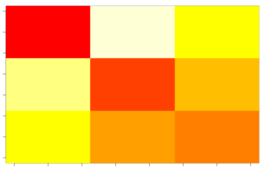
## fred 11 14 20 0.5555556image(1-fit$confusion[,3:1] / nn)